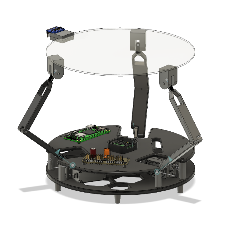
So I’ve been working on this neat little ball balancer for the last few weeks, since I saw it on YouTube, and thought it was pretty cool (basically how all of these projects start…). I knocked out a mechanical design in a week or so, and in less than two weeks, I had myself a fully viable platform that I could balance a ball on. Now came the problem of how exactly I’m going to do that.
I think the decision to use CV was rather obvious. It gave me the most freedom in designing the actual platform, as I would be constrained by dimensions of parts, like a capacitative touchscreen, or be limited to heavy metal bearings etc. The only real constraint was that I needed a transparent bottom platform. That was pretty easy to resolve, and so without a second thought, we’re using cameras!
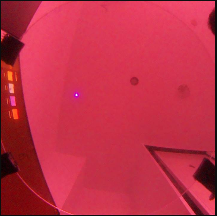
I’ve left most of the hardware details to its own post (that I will eventually get to..). I just wanted to cover the really janky CV loop that I’ve managed to implement. But I suppose it would be apt to cover the actual camera since it explains some of the stupid decisions I had to make later on. I kind screwed myself from the get-go, since I am just a moron. Basically when I was going to buy parts, I initially landed on the Raspberry Pi Camera Module 3, it was an obvious choice, easily integrated with the microcontroller + cheap. When I was about to add to cart, there were two options, a default, green PCB version, and a NoIR version, with a black PCB. I don’t know how this happened, but I bought the NoIR version, because cool black PCB, and I thought that was it, just a play on it being the French word for black (which I’m sure is still true, but less important than the other bit). Turns out NoIR, means it lacks an IR filter (duh!). And so now I have a camera which occasionally turns a brilliant shade of magenta whenever the white balance decides to not work. Fun!
The real kicker is that the original module, had too low an FOV, so I bought another camera module with a fisheye lense. At this point, I hadn’t yet understood that it was NoIR. And so I bought another NoIR camera. After already blowing a solid £30 on cameras, after I realised my mistake, there was no going back, and so I decided to fix it in software (not fun).
And with that in mind, I had to devise the requirements of my CV algorithm (on the fly of course). It had to be low latency, since my processing stack had me serving frames over HTTPS (implementing my own UDP stream is not something I want to do), and waiting for a response with the coordinates (did use UDP there), minimising processing time was somewhat important. Though in the end, I completely ignored this requirement. The more important ones were regarding the speed of the ball it can actually track. I wanted it to be able to track the ball even if its moving pretty fast across the screen. The hardest requirement was getting around the noise. I have a really cramped desk, and the frame of the balancer is really cluttered, plus living in the UK, the sun was setting at 3pm, till not too long ago, and so when I would work on it after school, the lighting would change drastically, and break my loop. And so my algorithm would have to be resilient to changes in lighting, and try and filter out noise as much as possible, whilst being fast.
Suffice to say, those are quite hefty requirements, especially for someone who’s never messed around with CV. And so I got stuck in. The first decision I had to make was on which broad algorithm to use. The two real options were the Hough Transform, and the Contour Detection.
Hough Transform#
So the Hough Transform is a pretty popular detection algorithm. It can be used to detect practically any shape from an image. In essence, the pixels of the image “vote” for the geometry that its part of. Essentially, instead of asking, “which pixels form a circle?”, it asks the pixel, if it were part of a circle, where it would be. Sounds counterintuitive, but bear with me.
The Hough Transform doesn’t work with pixels per se, but more with edges. And so we need to first pre-process the image with edge detection. Edge detection can be done with a variety of algorithms, but Canny is the one typically used in this context. It takes an image, converts it to grayscale, and to detect edges, it looks for rapid changes in intensity. A dark to light transition would indicate an edge. An image in a typical colourspace isn’t used since an edge could appear in any of the one channels, but not the other, but in a grayscale image, the edge is detected, regardless of hue.
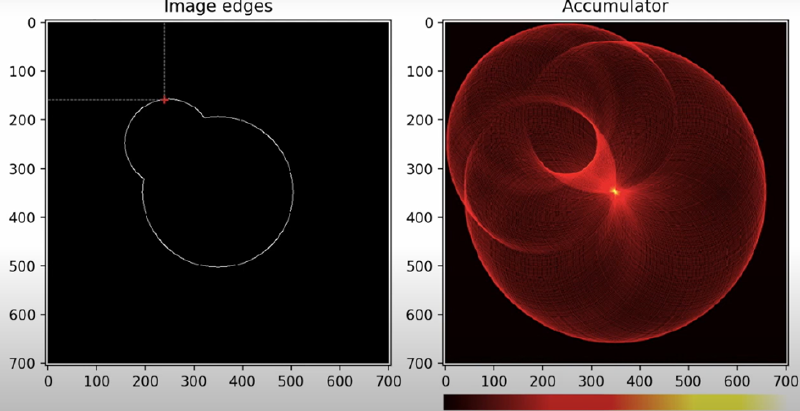
So we feed the algorithm an image with only the edges. And now the voting. For simplicities sake, lets say we have a fixed radius. For each point thats in the edge (represented as a 1 in the array), we fit a circle, of predetermined radius to it. How do you fit a circle with only one point and the radius? The simplest way is consider the radius at each angle \(\theta\) between \(0\) and \(\pi\), and compute the corresponding centres. You then define an accumulator array, and for each coordinate you generate, you update the accumulator’s corresponding coordinate index index by one. In the end you’ll have an array with a the “votes”, of all edge pixels. Then its a matter of looking at which centre has received the most “votes”, et voila, you have a circle!
Here is an example pipeline.
You take a raw image:
Then you convert it to grayscale using:
gray = cv.cvtColor(image, cv.COLOR_BGR2GRAY)giving you this:
edges = cv.Canny(gray, 50, 150, apertureSize=3)yielding:
With this in hand, you do some precomputing of all values of \(\cos{\theta}\) and \(\sin{\theta}\) to save having to do it each time, and then you fit centres for all points that are on the edges.
I couldn’t code a good looking accumulator animation after twiddling around with matplotlib and even manim for a bit, so here’s this cool graphic I found on the internet.
edgesProcessed = (edges/255).astype(np.uint8)
rows, cols = edgesProcessed.shape
accumulator = np.zeros((rows, cols),dtype=np.uint32) #set up accumulator
edgePixels = np.argwhere(edgesProcessed == 1)

thetas = np.deg2rad(np.arange(0, 360, 1)) #lists all angles of theta
cos = (radius*np.cos(thetas)).astype(int)  #lists all cosines of all thetas
sin = (radius*np.sin(thetas)).astype(int)  #lists all sines of all thetas

for y, x in edgePixels:

    a = x-cos # find all the x centres
    b = y-sin # find all the y centres

    indicies = (a>=0) & (a<cols) & (b>=0) & (b<rows)
    accumulator[b[indicies], a[indicies]] += 1

yCentre, xCentre = np.unravel_index(accumulator.argmax(), accumulator.shape)
print(xCentre, yCentre)
detected = image
cv2.circle(detected,(xCentre, yCentre), radius, (0,255,0), 2)
This implementation doesn’t take into account the fact that the radius is unknown. But some simple state management, or other techniques can be employed to sweep between a range, or select the most optimal radius.
This leaves you with this perfectly detected circle:
Pretty neat huh? The only real disadvantages of it, are that its computationally heavy, but since I’m processing the frames on my computer instead of the onboard computer, processing shouldn’t be a bottleneck. It does however struggle with moving objects, since it causes the ball to look more elliptical, and that skews the accumulator a tad bit. None of them are deal breakers, but inconveniences.
Contour Detection#
This algorithm is a fair amount more intuitive than the Hough Transform. A contour is defined as a curve that joins together continuous points (of the same type). Essentially it is the outline of an object. The entire pipeline, is very similar to that of Hough, you grayscale an image, do some edge detection, and you locate some contours. Locating them is pretty easy, again its just continuous sections of 1s. The problem comes with selecting which contour is the target. You can check the circularity of each detected contour using some basic maths:
$$ \frac{4\pi \cdot Area}{Perimeter^2} $$That would give us a number on a scale of 0 to 1. 1 means its a perfect circle. The thing is, with the noisy frame that I described earlier, this wouldn’t fly. I would likely flag multiple circles, all near 1 on the scale, and maybe of similar radius too, making it hard to differentiate. Of course this issue is a problem with pure Hough as well. And as such, the majority of my pipeline is filtering and accounting for noise. I took multiple approaches, some novel, some pretty cool.
My Janky Pipeline#
I’m not quite sure I bothered outlining contour detection. Sure I could have used it for my algorithm, but I would have to do a lot more of the grunt work than if I used Hough, which I did. I overcame the performance overhead of the Hough Transform by using “edge computing”. Thats just a hype term I threw out, I’m not entirely confident that its totally accurate. I’m off-loading the processing to my computer, by serving the frames over HTTPS (using Flask), and then awaiting a response over UDP. If you understand what that is, you’ll realise how stupid that is, using UDP for the actual streaming would be so much smarter, since I wouldn’t have to wait for a handshake each frame, but implementing my own UDP stream for my frames was too complicated, and I didn’t want to relearn another library to do that, since I had already implemented it with Flask, and so we stick with this janky architecture.
Pre-processing#
I start by defining a static Region of Interest (RoI). This crops out the part of the frame that I’m not interested in. I define my RoI with simple rectangles, but you can totally use more complicated shapes.
maskRoi = np.zeros((height, width), dtype=np.uint8)  # static roi to define area to ignore
cv2.rectangle(maskRoi, (vertBar[0], vertBar[1]), (vertBar[0] + vertBar[2], vertBar[1] + vertBar[3]), 255, -1)
cv2.rectangle(maskRoi, (horizBar[0], horizBar[1]), (horizBar[0] + horizBar[2], horizBar[1] + horizBar[3]), 255, -1)
Also another smarter use of RoI is a dynamic RoI. Assuming that I have locked onto a target with a certain confidence, I define a smaller square surrounding the ball. For future frames, I will only process that area, instead of the entire area. This reduces processing time, since we’re searching a smaller area, and it improves accuracy since the algorithm can’t get distracted by some random artefacts in some obscure corner of the frame.
To actually get rid of the parts of the frame we don’t need, we do a bitwise and. Only pixels in the defined RoI, and pixels in the frame stay, effectively purging all pixels outside of our RoI.
maskedFrame = cv2.bitwise_and(maskRoi, frame) # example usageWe first use a colour mask to rid ourselves of colours outside our wanted range.
combinedMask = cv2.bitwise_and(maskRoi, colourMask)And now we convert the frame into grayscale.
maskedGray = cv2.bitwise_and(grayFrame, combinedMask)And then apply a blur.
blurredFrame = cv2.GaussianBlur(maskedGray, (9, 9), 0)The type of blur used is a point of contention. The two main blurs are Median and Gaussian. I won’t get into the details, but the Median blur preserves edges better than Gaussian does. It also gets rid of “salt and pepper” noise, as in that of small specks. Gaussian blur is more general purpose, and does ruin the definition of edges, though it is better at cleaning raw sensor noise.
For my application, it would be more suitable to use a Median blur since its edge preservation is advantageous for faster moving objects. I don’t quite remember when in the development cycle I switched to Gaussian from Median, but I haven’t switched back since my CV pipeline is working really well now, and you know the saying.. if it ain’t broke, don’t fix it. I’m using a relatively large kernel size (size of the array of pixels it take in batches to blur). I settled on a relatively larger kernel size, you should probably go for a lower one, but the heavier blur is useful to get rid of as much noise as possible.
Processing#
I don’t actually have to implement my own Hough Circle Transform algorithm, the OpenCV library has an implementation thats leagues better than something I could achieve.
detectedCircles = cv2.HoughCircles(blurredFrame, cv2.HOUGH_GRADIENT, 1.2, 60, param1=50, param2=15, minRadius=75, maxRadius=100)The function takes in its fair share of parameters. The most important ones are:
dp = 1.2
minDist = 60
param1 = 50
param2 = 15
minRadius = 75
maxRadius = 100- dp is the inverse ratio between the accumulator resolution to the image resolution. Being inverse, a higher value means lower resolution of the accumulator, making the processing time faster. With my hardware I could get away with a 1.0, of perhaps even upscaling it, but I started with 1.2, it works, and so it stays.
- minDist: Define the minimum distance between detected circles. It has to be relatively low for me, since the ball does move a fair amount
- param1: Its the threshold for the Canny Edge detector.
- param2: The accumulator threshold. Probably the most important value to tune. Sort of the circularity tuning. A lower value means it accepts more elliptical shape, and a higher value means its looking for a well defined circle. I have it relatively low, since when the ball moves, its more of an ellipse than a circle. Also weird lighting cuts parts of the circle off, even when stationary.
- minRadius and maxRadius: These two are relatively straightforward, they define the smallest and largest circles it can detect.
Post-processing#
Colour Thresholding#
Now that we have our detected circles, we need to validate its what we wanted. I need this to be rather robust, due to the high amount of noise in my system. I choose to use are rather novel colour thresholding approach. I manually define a HSV range for my ball, and an acceptance threshold depending on the lighting.
I then swatch the pixels in the centre of the detected ball, for their colour, in a predefined radius. I calculate what percent of HSV is in my range, and if its above my threshold, I accept that detection.
Exponential Moving Average (EMA)#
Since we’re processing at a discrete frame rate, we’re essentially sampling the coordinates of the ball a set number of times a second. In reality of course, the ball isn’t teleporting between points at a certain frame rate. To account for that in our data, we use EMA, which smooths our the detected coordinates.
The formula:
$$ S_{t}= \alpha \cdot A_{t} + (1-\alpha) \cdot S_{t-1} $$Where \(S_t\) = smoothed position, \(\alpha\) = dynamic alpha (how much to trust the old data), \(A_t\) is the raw coordinates, and \(S_{t-1}\) is the old smoothed average.
You tune the alpha to trust the old data more or less, and it results in a smoothed out value for the centre of our ball.
emaCenter = (dynamicAlpha * newCenter) + ((1 - dynamicAlpha) * emaCenter)Other stuff#
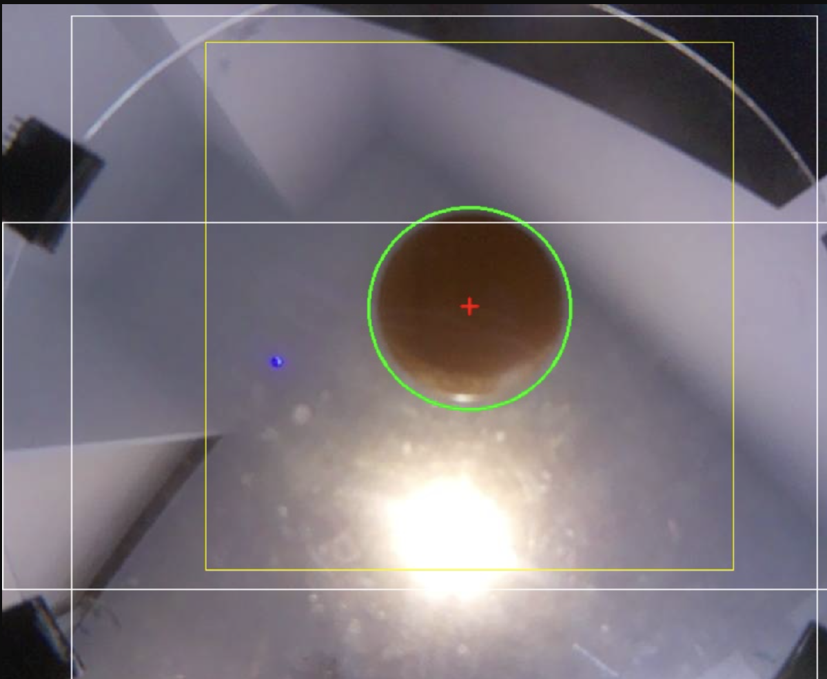
Now we have all the important bits of post-processing done, we just calculate the velocity based on old data, and package it into a nice list, and we send it off to our ball balancer to deal with. We also do some fancy annotations onto our frame, with the RoIs, and a circle highlighting the detected ball, and a marker for its centre.
The remaining 80% of the code in my CV script is just supporting architecture, doing stuff like handling missing frames, packaging and sending data, ensuring we’re being served frames, etc. The boring stuff.
This is my entire function (with the supporting architecture):
def processFrame(frame):
    global ballCenter, lastKnownCenter, missingFrames, emaCenter, isLocked, velocity, lastFrameTime, relCenter, latestBlurred, lastRawCenter
    currentTime = time.time()
    deltaTime = currentTime - lastFrameTime
    lastFrameTime = currentTime
    height, width = frame.shape[:2]

    maskRoi = np.zeros((height, width), dtype=np.uint8)  # static roi to define area to ignore
    cv2.rectangle(maskRoi, (vertBar[0], vertBar[1]), (vertBar[0] + vertBar[2], vertBar[1] + vertBar[3]), 255, -1)
    cv2.rectangle(maskRoi, (horizBar[0], horizBar[1]), (horizBar[0] + horizBar[2], horizBar[1] + horizBar[3]), 255, -1)

    if isLocked and ballCenter is not None:
        winSize = 500  # somewhat large
        x1, y1 = max(0, ballCenter[0] - winSize // 2), max(0, ballCenter[1] - winSize // 2)
        x2, y2 = min(width, ballCenter[0] + winSize // 2), min(height, ballCenter[1] + winSize // 2)
        searchMask = np.zeros((height, width), dtype=np.uint8)
        cv2.rectangle(searchMask, (x1, y1), (x2, y2), 255, -1)
        maskRoi = cv2.bitwise_and(maskRoi, searchMask)
        cv2.rectangle(frame, (x1, y1), (x2, y2), (0, 255, 255), 1)

    hsvFrame = cv2.cvtColor(frame, cv2.COLOR_BGR2HSV)
    colourMask = cv2.inRange(hsvFrame, hsvLow, hsvHigh)
    kernel = np.ones((7, 7), np.uint8)
    colourMask = cv2.morphologyEx(colourMask, cv2.MORPH_CLOSE, kernel)
    colourMask = cv2.dilate(colourMask, kernel, iterations=1)

    combinedMask = cv2.bitwise_and(maskRoi, colourMask)
    grayFrame = cv2.cvtColor(frame, cv2.COLOR_BGR2GRAY)
    maskedGray = cv2.bitwise_and(grayFrame, combinedMask)
    blurredFrame = cv2.GaussianBlur(maskedGray, (9, 9), 0)

    _, encodedBlurred = cv2.imencode(".jpg", blurredFrame)
    with frameLock:
        latestBlurred = encodedBlurred.tobytes()

    detectedCircles = cv2.HoughCircles(blurredFrame, cv2.HOUGH_GRADIENT, 1.2, 60, param1=50, param2=15, minRadius=75, maxRadius=100)
    detectedThisFrame = False

    if detectedCircles is not None:
        detectedCircles = np.uint16(np.around(detectedCircles))
        for circle in detectedCircles[0, :]:
            centerX, centerY, radius = circle
            if 0 <= centerY < height and 0 <= centerX < width:
                sampleRadius = 20
                sy1, sy2 = max(0, centerY - sampleRadius), min(height, centerY + sampleRadius)
                sx1, sx2 = max(0, centerX - sampleRadius), min(width, centerX + sampleRadius)
                if sy2 > sy1 and sx2 > sx1:
                    sampleRegion = hsvFrame[sy1:sy2, sx1:sx2]
                    avgHsv = [round(x, 1) for x in cv2.mean(sampleRegion)[:3]]
                    orangeMask = cv2.inRange(sampleRegion, hsvLow, hsvHigh)
                    orangePercent = np.count_nonzero(orangeMask) / orangeMask.size

                    if orangePercent > threshold:
                        print(f"Lock - HSV: {avgHsv} Match: {orangePercent * 100:.1f}%")
                        newCenter = np.array([centerX, centerY], dtype=float)
                        detectedThisFrame = True

                        if lastRawCenter is not None and deltaTime > 0:
                            rawDiff = newCenter - lastRawCenter
                            distMoved = np.linalg.norm(rawDiff)

                            if distMoved < 4.0:
                                rawDiff = np.array([0.0, 0.0])

                            instantVelocity = rawDiff / deltaTime
                            instantSpeed = np.linalg.norm(instantVelocity)

                            currentSpeed = np.linalg.norm(velocity)
                            if (instantSpeed > 25.0) or (currentSpeed > 10.0 and instantSpeed > 5.0):
                                velocity = (0.92 * velocity) + (0.08 * instantVelocity)
                            else:
                                velocity = velocity * 0.5
                                if np.linalg.norm(velocity) < 1.0:
                                    velocity = np.array([0.0, 0.0])

                        lastRawCenter = newCenter.copy()

                        if emaCenter is None:
                            emaCenter = newCenter
                        else:
                            currentSpeed = np.linalg.norm(velocity)
                            dynamicAlpha = np.clip(0.15 + (currentSpeed / 2000), 0.15, 0.6)
                            emaCenter = (dynamicAlpha * newCenter) + ((1 - dynamicAlpha) * emaCenter)

                        ballCenter = (int(emaCenter[0]), int(emaCenter[1]))
                        lastKnownCenter = (int(newCenter[0]), int(newCenter[1]))
                        missingFrames, isLocked = 0, True
                        cv2.circle(frame, (centerX, centerY), radius, (0, 255, 0), 2)
                        break

    if not detectedThisFrame:
        missingFrames += 1
        lastRawCenter = None
        if isLocked and missingFrames > 3:
            isLocked = False
            ballCenter = None
        if missingFrames > 5:
            emaCenter, velocity = None, np.array([0.0, 0.0])

    if emaCenter is not None:
        posX = float(emaCenter[0] - width / 2)
        posY = float(-(emaCenter[1] - height / 2))
        relCenter = (posX, posY)

        outputVel = velocity.tolist()
        if np.linalg.norm(velocity) < 5.0:
            outputVel = [0.0, 0.0]

        try:
            packet = json.dumps({
                "x": round(posX, 2),
                "y": round(posY, 2),
                "det": True,
                "vel": [round(v, 2) for v in outputVel]
            }).encode()
            sock.sendto(packet, (targetIP, port))
        except Exception as e:
            print(f"UDP Error: {e}")
    else:
        relCenter = None
        try:
            packet = json.dumps({"det": False}).encode()
            sock.sendto(packet, (targetIP, port))
        except:
            pass

    cv2.rectangle(frame, (vertBar[0], vertBar[1]), (vertBar[0] + vertBar[2], vertBar[1] + vertBar[3]), (255, 255, 255),
                  1)  # annotations
    cv2.rectangle(frame, (horizBar[0], horizBar[1]), (horizBar[0] + horizBar[2], horizBar[1] + horizBar[3]),
                  (255, 255, 255), 1)
    if emaCenter is not None:
        cv2.drawMarker(frame, (int(emaCenter[0]), int(emaCenter[1])), (0, 0, 255), cv2.MARKER_CROSS, 15, 2)
    return frame
I apologise for my obscenely long function.. I was going to refactor it eventually..
The other helpers to aid with streaming and whatnot can be found at my GitHub.
Here’s a cool little demonstration of it doings its thing (it may just be a placeholder for now..)!
Thanks for reading!